Reinforcement Learning for Lane Following
In this tutorial, you will learn how to use the Reinforcement Learning algorithm Proximal Policy Optimization (PPO) to train a lane following policy.
Introduction: Why Reinforcement Learning?
Classical control methods rely on explicitly designed mathematical models and control theory principles. They are highly interpretable, stable, and computationally efficient, making them ideal for simple, well-understood systems. However, they require significant domain expertise to tune and often struggle with high-dimensional observations like camera images or complex, changing environments where the system dynamics are hard to model perfectly.
Behavior cloning, or imitation learning, bypasses the need for manual controller design by training a neural network to mimic expert demonstrations. This approach is sample-efficient and can handle complex inputs like visual data, leveraging standard supervised learning techniques. The downside is that the agent is limited by the quality of the expert data and cannot exceed the expert's performance. It also suffers from distribution shift, where small errors compound over time, leading the agent into states it has never seen and does not know how to recover from.
Reinforcement learning (RL) addresses these limitations by allowing an agent to learn through trial and error interactions with the environment, optimizing for long-term cumulative rewards. Unlike classical control, it can handle complex sensory inputs without explicit models, and unlike behavior cloning, it can discover novel strategies that exceed human performance. While RL is computationally expensive and can be unstable to train, it is powerful for solving complex tasks where expert data is unavailable or where the optimal strategy is unknown.
RL problems are typically formulated as Markov Decision Processes (MDPs). A Markov Decision Process is a mathematical framework for modeling sequential decision-making problems. It consists of a set of states, a set of actions, a transition probability function, and a reward function. The agent's goal is to learn a policy that maximizes the expected cumulative reward.
Components of an MDP:
-
State (s): Current observation of the environment
- Example: Camera image showing the track ahead
- Can be fully observable (you see everything) or partially observable (you only see recent history)
-
Action (a): What the agent can do
- Example:
[steering_angle, throttle]for an autonomous vehicle - Can be discrete (left/right/straight) or continuous (real-valued steering angle)
- Example:
-
Reward (r): Feedback signal indicating how good the current state-action pair is
- Example: \(+1.0\) for staying on track, \(-10.0\) for crashing, \(+100.0\) for completing a lap
- Critically, the reward function determines what the agent learns!
-
Policy (π): The agent's strategy - a function mapping states to actions
- Deterministic: \(a = \pi(s)\) (always same action for same state)
- Stochastic: \(a \sim \pi(\cdot|s)\) (samples action from a probability distribution)
-
Value Functions: Estimate how good states or actions are
- V(s): Expected cumulative reward from state \(s\) following policy \(\pi\)
- Q(s,a): Expected cumulative reward from taking action \(a\) in state \(s\), then following \(\pi\)
The RL Loop:
The interaction between the agent and the environment happens in a continuous cycle:
graph LR
    Agent[Agent] -- Action a_t --> Env[Environment]
    Env -- State s_{t+1} --> Agent
    Env -- Reward r_t --> Agent
    style Agent fill:#f9f,stroke:#333,stroke-width:2px
style Env fill:#bbf,stroke:#333,stroke-width:2px- Observation: At time step \(t\), the agent observes the current state of the environment, \(s_t\).
- Decision: The agent's policy \(\pi\) selects an action \(a_t\) based on this observation. This can be deterministic or sampled from a distribution.
- Action: The agent executes action \(a_t\) in the environment.
- Transition: The environment changes in response to the action, transitioning to a new state \(s_{t+1}\).
- Feedback: The environment provides a reward signal \(r_t\), indicating the immediate quality of the action.
- Learning: The agent uses the experience tuple \((s_t, a_t, r_t, s_{t+1})\) to update its policy, aiming to maximize future cumulative rewards.
During training, the agent gathers many of these interaction tuples into trajectories. These trajectories are then processed by the algorithm to compute advantage estimates and perform policy updates. Repeating this loop over many episodes gradually improves the policy's performance.
Types of RL Algorithms
- Value-based: Learn \(Q(s,a)\), then derive policy (e.g., Q-learning, DQN)
- Policy-based: Directly learn \(\pi(\cdot|s)\) (e.g., REINFORCE, PPO)
- Actor-Critic: Combine both - learn both policy and value function (e.g., PPO, A3C)
On-policy vs Off-policy:
- On-policy (PPO): Learn from data collected by current policy. Must collect fresh data each update.
- Off-policy (DQN, SAC): Can learn from data collected by old policies. Can reuse past experience.
Why PPO?
PPO is particularly well-suited for continuous control tasks (like autonomous racing) because:
-
Handles continuous actions naturally: Unlike value-based methods that require either discretization of actions or more expensive workarounds, PPO directly optimizes the actor.
-
Stable learning: The clipping mechanism prevents the policy from changing too drastically, which is crucial for continuous control where small changes can have large effects.
-
Sample efficient (for on-policy): While not as efficient as off-policy methods, PPO is more sample efficient than simpler policy gradient methods like REINFORCE.
-
Works with high-dimensional observations: The actor-critic architecture with neural networks can process camera images, lidar, etc.
-
Industry standard: Widely used in practice (OpenAI, DeepMind, robotics companies) with proven results.
Trade-offs compared to other RL methods:
- vs DQN: PPO handles continuous actions, but DQN is off-policy (more sample efficient)
- vs SAC: SAC is off-policy (more sample efficient), but PPO is simpler and more stable
- vs TRPO: PPO is simpler (no second-order optimization), but slightly less stable theoretically
Tutorial Steps
First, setup the simulation environment on your computer or a lab machine.
Note: once you have the simulation environment set up, you may need to run the
checkout.shscript in~/roboracer_ws/scriptsto pull the latest changes for the simulation repository. If theDockerfilehas changed, be sure to run./container buildto rebuild the container.
1. Training a PPO Policy
Once your simulation environment is ready, you can train a PPO policy by running the rl_ppo tmux config or by running (in a ./container shell).
First, start the vnc server: vnc.
Then, run the simulator:
cd ~/roboracer_ws/simulator
uv run python src/algorithms/ppo_pufferlib.py \
  --random-spawn \
  --random-spawn-max-cte-offset 0.8 \
  --random-spawn-max-rotation-offset 10.0 \
  --num-envs 1 \
  --total-timesteps 2000000 \
  --visualize \
  --env-name donkey-roboracingleague-track-v0
Connect to your lab machine using the TurboVNC viewer and you should see the simulator running.
Note that while the total timesteps is set to 2M, you can stop the training when the policy achieves the desired level of performance.
Note: to train faster, you can try use
--num-envs 4to use 4 environments in parallel. There are many options you can use to modify the training behavior of the PPO policy in theppo_pufferlib.pyscript. Inspect theppo_pufferlib.pyscript or run the help command to see the available options:uv run python src/algorithms/ppo_pufferlib.py --help.
The environments you can try are:
- donkey-roboracingleague-track-v0
- donkey-avc-sparkfun-v0
- donkey-warehouse-v0
- donkey-circuit-launch-track-v0
Note: Only the roboracingleague and circuitlaunch environments have been tested.
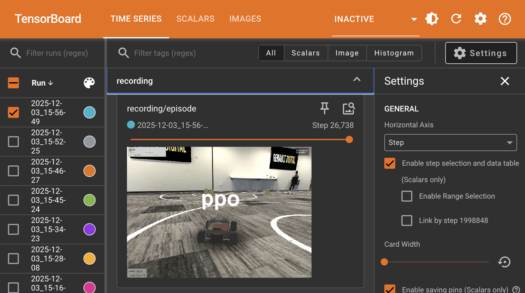
You'll first see the simulator window open, then you'll see the visualization window open.
- The simulator window shows a 3rd person view of the car.
-
The visualization window shows the car's camera view, the steering and throttle values, and the reward.
As the model trains, you should see the performance of the car improve. For example, here is my car at step 37:
Update 37/97 | Step 75776 | SPS: 19
  CTE: 2.364 | Speed: 2.91 | Collisions: 0.00%
  Termination: off_track: 4 | car_fully_crossed: 2
  PG Loss: -0.0851 | V Loss: 120.2045
  Entropy: 1.5089 | KL: 0.7787
As you train, the associated data will be saved in 3 folders within the output directory. Within each of the following folders, a new run folder is created corresponding to the time at which the run was started:
models: Contains the latest checkpoint of the policy.tensorboard: Contains the training metrics.videos: Contains the videos of the car following the lane.
As the policy begins to train, launch tensorboard to view the training metrics:
Note: uv commands should be run outside the container
cd ~/roboracer_ws/simulator
uv run tensorboard --logdir ./output/tensorboard/ --host 0.0.0.0
And open http://localhost:6006 in your browser to view the training metrics.
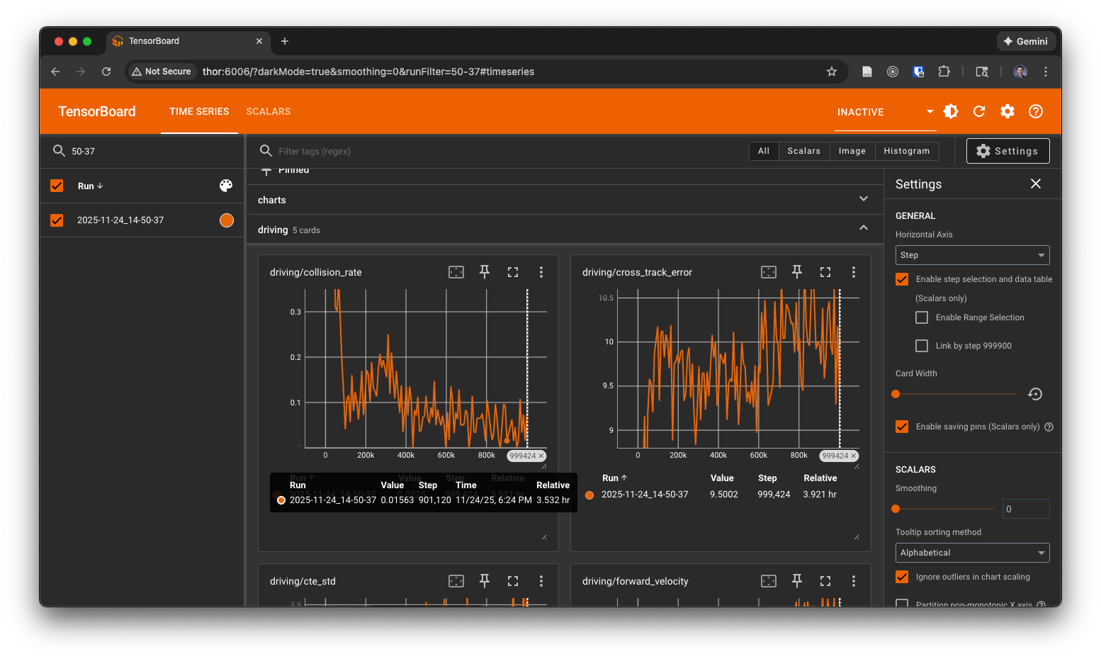
You'll also be able to view the videos of the car in tensorboard:
Lab Notebook
- Explore the available evaluation metrics and losses in tensorboard and record your observations in your lab notebook.
- Identify the most important losses and metrics, explain how they are related to the process of learning the policy.
- Watch training for a while and write down your observations of the policy's behavior.
After a period of time, you should start to see the car follow the lane and make it further along the race track.
Note: You can train for a large number of timesteps, however, your cars performance may not improve, and may actually decrease at a certain point. Use the videos saved to disk along with measures recorded to tensorboard to monitor the car's behavior and determine when to stop training and which model weights to test for the best performance in the next steps.
Lab Notebook
- Record the name of the machine you used and the command you ran to train the model.
- As training progresses, record your observations of the policy's behavior in your lab notebook.
- Does your policy's performance increase and then decrease? If so, why do you think this happens?
Resuming Training
If you are satisfied with the performance of the policy, you can stop the training. Or if you stop training and want to resume later, you can use the same command, but also include the --model-path flag with the checkpoint to resume training from that checkpoint, for example:
cd ~/roboracer_ws/simulator
uv run python src/algorithms/ppo_pufferlib.py \
  --random-spawn \
  --random-spawn-max-cte-offset 0.8 \
  --random-spawn-max-rotation-offset 10.0 \
  --num-envs 1 \
  --total-timesteps 2000000 \
  --visualize \
  --env-name donkey-roboracingleague-track-v0 \
  --model-path ./output/models/2025-12-03_15-56-49/update_217.pt
You'll notice that when you resume training, a new run folder is created corresponding to the time at which the run was started. The model checkpoints and tensorboard logs are also saved in the new run folder. Be sure to write down a note with both the old run name (2025-12-03_15-56-49) and the new run name (2025-12-04_10-03-27) and the associated training commands so that someone else could reproduce your results.
============================================================
Starting PPO training with PufferLib
============================================================
Total timesteps: 2000000
Num environments: 1
Steps per rollout: 2048
Batch size: 2048
Minibatch size: 64
Device: cuda
Tensorboard logs: ./output/tensorboard/2025-12-04_10-03-27
Model checkpoints: ./output/models/2025-12-04_10-03-27
============================================================
Replaying a Pretrained Policy
To give you an idea of how well your policy might perform, I trained a policy until around step 200 and the car was able to make a complete lap:
If you would like to replay this trained policy, download the model weights (update_217.pt) to your ~/roboracer_ws/simulator/output/models/2025-12-03_15-56-49 folder (which you will need to create) and run the following command:
cd ~/roboracer_ws/simulator
uv run python src/algorithms/ppo_pufferlib.py \
  --playback \
  --visualize \
  --env-name donkey-roboracingleague-track-v0 \
  --model-path ./output/models/2025-12-03_15-56-49/update_217.pt
You'll see a summary of the performance once all 10 playback episodes are complete.
============================================================
PLAYBACK COMPLETE - AGGREGATE STATISTICS
============================================================
Total Episodes: 10
Total Steps: 3915
Total Time: 197.25s
Average SPS: 19
============================================================

Lap Performance:
  Total Laps Completed: 2
  Avg Laps per Episode: 0.20
  Episodes with Laps: 1/10
  Best Lap Time: 28.71s
  Mean Lap Time: 28.71s ± 0.00s
  Worst Lap Time: 28.71s

Driving Performance:
  Cross-Track Error: Mean=1.767, Std=0.774, Min=0.216, Max=2.266
  Speed: Mean=1.67, Std=0.91, Min=0.00, Max=2.65
  Forward Velocity: Mean=1.68, Std=0.92

Collision Statistics:
  Collision Rate: 0.0%
  Episodes with Collisions: 0/10
============================================================
2. Testing the Policy
Once the policy is trained, you can test it by running the following command, replace 2025-11-21_14-10-20 with the name of your run folder and ppo_donkey_final.pt with the model checkpoint you want to test:
cd ~/simulator
uv run python src/algorithms/ppo_pufferlib.py \
  --playback \
  --visualize \
  --env-name donkey-roboracingleague-track-v0 \
  --model-path ./output/models/2025-11-21_14-10-20/ppo_donkey_final.pt
Note: be sure to use the
--env-name donkey-roboracingleague-track-v0flag, which matches the environment name you used in training to see how well your policy performs with the "in distribution" environment.
Once the 10 runs complete, you'll see something like the following in your terminal:
Lab Notebook
- Observe how well your policy performs with the "in distribution" environment.
- Record the training command and the evaluation command in your lab notebook.
- In a "results" section, record your subjective observations of the policy's performance.
- Include a screenshot from the run.
Now, test how well your policy performs in an environment that it was not trained on, by running:
cd ~/simulator
uv run python src/algorithms/ppo_pufferlib.py \
  --playback \
  --visualize \
  --env-name donkey-circuit-launch-track-v0 \
  --model-path ./output/models/2025-11-21_14-10-20/ppo_donkey_final.pt
Lab Notebook
- Observe how well your policy performs with the "out of distribution" environment.
- Record the training command and the evaluation command in your lab notebook.
- In a "results" section, record your subjective observations of the policy's performance.
- Include a screenshot from the run.
3. Improving the Policy
Many different techniques can be used to improve the policy. Here are a few examples:
Curriculum Learning
Curriculum learning is a technique that gradually increases the difficulty of the task as the policy learns. We'll use this technique to gradually increase the speed of the car as the policy learns.
uv run python src/algorithms/ppo_pufferlib.py \
  --curriculum-learning \
  --curriculum-initial-speed 0.25 \
  --curriculum-target-speed 2.5 \
  --num-envs 1 \
  --total-timesteps 2000000 \
  --visualize \
  --env-name donkey-roboracingleague-track-v0
Varying the starting position
This strategy is included in the default training command as its necessary to learn a reasonablly performant policy.
uv run python src/algorithms/ppo_pufferlib.py \
  --random-spawn \
  --random-spawn-max-cte-offset 0.8 \
  --random-spawn-max-rotation-offset 10.0 \
  --num-envs 1 \
  --total-timesteps 2000000 \
  --visualize \
  --env-name donkey-roboracingleague-track-v0
Reward Shaping
Note: The reward calculation is defined in
src/gym_donkeycar/envs/donkey_sim.py. Feel free to use the flags here or directly modify the reward calculation in the source code.
The default reward calulation encourages the robot to move quickly and stay close to the centerline of the track, which we call Cross Track Error (CTE). The reward is calculated as the product of the speed reward and the CTE reward:
reward = (1.0 - |CTE|/max_cte) * speed_reward
Alternatively, you can change the reward from the product of the speed reward and the CTE reward to a linear combination of the reward elements. This is done by setting the --reward-lin-combination flag and the weights of the reward elements. For example, to make the centering reward twice as important as the speed reward, you would set:
  --reward-lin-combination \
  --reward-speed-weight 1.0 \
  --reward-centering-weight 2.0 \
There are other elements of the reward you can change.
- Cross Track Error (CTE)
You can try to adjust how the CTE error is calculated. Instead of just using the linear distance from the car's center to the centerline of the track, we can use a 5-point spline to define the reward. For example, if we set:
  --centering-setpoint-x 0.4 \
  --centering-setpoint-y 0.7 \
This will keep the reward high close to the centerline of the track, but make it drop off more quickly as the car moves further away from the centerline.
- Reward Distance
--reward-distance-weight controls the weight of the distance reward. A higher weight will increase the reward when the car travels further down the track.
- Done Penalty
--reward-done-penalty controls the penalty when the car collides with the track or goes off the track. A higher penalty will make the car avoid collisions and going off the track.
Performing Smoother Actions
You can enable action smoothing to prevent the car from making jerky movements. This is useful for transferring the policy to the real world.
--action-smoothing: Enable action smoothing (default: False).--action-smoothing-sigma: Controls the smoothness of the actions. A higher value will make the actions smoother. (default: 1.0)--action-history-len: The number of past actions to use for smoothing. (default: 120)--min-throttle: The minimum throttle value to apply. (default: 0.0)
Lab Notebook
- Run another training run using some of the options above.
- Record the training command.
- Observe your new policy and record your subjective observations of the policy's performance.
- Has it improved? If so, how?
- Does it generalize to an out-of-distribution environment?
- How could you improve it further?
Troubleshooting
- Missing display
If you see a parsing error, like this:
[docker]:ntsoi@thor:~/roboracer_ws/simulator$ uv run python src/algorithms/ppo_pufferlib.py --random-spawn --random-spawn-max-cte-offset 0.8 --random-spawn-max-rotation-offset 10.0 --num-envs 1 --total-timesteps 200000000 --visualize --env-name donkey-roboracingleague-track-v0
/home/ntsoi/.venv/lib/python3.14/site-packages/torch/cuda/__init__.py:63: FutureWarning: The pynvml package is deprecated. Please install nvidia-ml-py instead. If you did not install pynvml directly, please report this to the maintainers of the package that installed pynvml for you.
  import pynvml  # type: ignore[import]
Gym has been unmaintained since 2022 and does not support NumPy 2.0 amongst other critical functionality.
Please upgrade to Gymnasium, the maintained drop-in replacement of Gym, or contact the authors of your software and request that they upgrade.
See the migration guide at https://gymnasium.farama.org/introduction/migration_guide/ for additional information.
Creating 1 parallel environments...
Random spawn enabled: lateral offset ±0.8m, rotation offset ±10.0°
Reward weights: speed=1.0, centering=1.0, distance=0.0
Done penalty: -1.0
Reward linear combination: False
Centering reward setpoints: x=0.3, y=0.8
Launching simulator with command:
  ./simulator/build/linux/sim.x86_64 --scene roboracingleague_1 --port 9091 --host 0.0.0.0 -logfile -
Simulator process started (PID: 134)
Logging simulator output to: /home/ntsoi/roboracer_ws/simulator/logs/sim_output_9091_1764700302.log
Traceback (most recent call last):
  File "/home/ntsoi/roboracer_ws/simulator/src/algorithms/ppo_pufferlib.py", line 1061, in <module>
    main()
    ~~~~^^
  File "/home/ntsoi/roboracer_ws/simulator/src/algorithms/ppo_pufferlib.py", line 1051, in main
    trainer = PPOTrainer(config)
  File "/home/ntsoi/roboracer_ws/simulator/src/algorithms/ppo_pufferlib.py", line 385, in __init__
    self.envs = make_vectorized_env(
                ~~~~~~~~~~~~~~~~~~~^
        env_name=config.env_name,
        ^^^^^^^^^^^^^^^^^^^^^^^^^
    ...<4 lines>...
        env_config=env_config,
        ^^^^^^^^^^^^^^^^^^^^^^
    )
    ^
  File "/home/ntsoi/roboracer_ws/simulator/src/algorithms/pufferlib_wrapper.py", line 194, in make_vectorized_env
    vecenv = pufferlib.vector.make(
        env_creators,
    ...<3 lines>...
        num_envs=num_envs,
    )
  File "/home/ntsoi/.venv/lib/python3.14/site-packages/pufferlib/vector.py", line 708, in make
    return backend(env_creators, env_args, env_kwargs, num_envs, **kwargs)
  File "/home/ntsoi/.venv/lib/python3.14/site-packages/pufferlib/vector.py", line 61, in __init__
    self.driver_env = env_creators[0](*env_args[0], **env_kwargs[0])
                      ~~~~~~~~~~~~~~~^^^^^^^^^^^^^^^^^^^^^^^^^^^^^^^
  File "/home/ntsoi/roboracer_ws/simulator/src/algorithms/pufferlib_wrapper.py", line 173, in make_env
    return pufferlib.emulation.GymnasiumPufferEnv(env_creator=env_creator, **kwargs)
           ~~~~~~~~~~~~~~~~~~~~~~~~~~~~~~~~~~~~~~^^^^^^^^^^^^^^^^^^^^^^^^^^^^^^^^^^^
  File "/home/ntsoi/.venv/lib/python3.14/site-packages/pufferlib/emulation.py", line 143, in __init__
    self.env = make_object(env, env_creator, env_args, env_kwargs)
               ~~~~~~~~~~~^^^^^^^^^^^^^^^^^^^^^^^^^^^^^^^^^^^^^^^^
  File "/home/ntsoi/.venv/lib/python3.14/site-packages/pufferlib/emulation.py", line 443, in make_object
    return object_creator(*creator_args, **creator_kwargs)
  File "/home/ntsoi/roboracer_ws/simulator/src/algorithms/pufferlib_wrapper.py", line 167, in env_creator
    env = start_sim(env_name=env_name, port=port, conf=conf)
  File "/home/ntsoi/roboracer_ws/simulator/src/utils/sim_starter.py", line 314, in start_sim
    proc, port = launch_simulator(scene=scene, sim_path=sim_path, port=port, debug=debug)
                 ~~~~~~~~~~~~~~~~^^^^^^^^^^^^^^^^^^^^^^^^^^^^^^^^^^^^^^^^^^^^^^^^^^^^^^^^
  File "/home/ntsoi/roboracer_ws/simulator/src/utils/sim_starter.py", line 233, in launch_simulator
    line = proc.stdout.readline()
  File "<frozen codecs>", line 325, in decode
UnicodeDecodeError: 'utf-8' codec can't decode byte 0xf6 in position 78: invalid start byte
[W1202 18:31:44.236492559 AllocatorConfig.cpp:28] Warning: PYTORCH_CUDA_ALLOC_CONF is deprecated, use PYTORCH_ALLOC_CONF instead (function operator())
Then, check the log file, like so:
[docker]:ntsoi@thor:~/roboracer_ws/simulator$ cat  /home/ntsoi/roboracer_ws/simulator/logs/sim_output_9091_1764700302.log
[UnityMemory] Configuration Parameters - Can be set up in boot.config
    "memorysetup-allocator-temp-initial-block-size-main=262144"
    "memorysetup-allocator-temp-initial-block-size-worker=262144"
    "memorysetup-bucket-allocator-granularity=16"
    "memorysetup-bucket-allocator-bucket-count=8"
    "memorysetup-bucket-allocator-block-size=4194304"
    "memorysetup-bucket-allocator-block-count=1"
    "memorysetup-main-allocator-block-size=16777216"
    "memorysetup-thread-allocator-block-size=16777216"
    "memorysetup-gfx-main-allocator-block-size=16777216"
    "memorysetup-gfx-thread-allocator-block-size=16777216"
    "memorysetup-cache-allocator-block-size=4194304"
    "memorysetup-typetree-allocator-block-size=2097152"
    "memorysetup-profiler-bucket-allocator-granularity=16"
    "memorysetup-profiler-bucket-allocator-bucket-count=8"
    "memorysetup-profiler-bucket-allocator-block-size=4194304"
    "memorysetup-profiler-bucket-allocator-block-count=1"
    "memorysetup-profiler-allocator-block-size=16777216"
    "memorysetup-profiler-editor-allocator-block-size=1048576"
    "memorysetup-temp-allocator-size-main=4194304"
    "memorysetup-job-temp-allocator-block-size=2097152"
    "memorysetup-job-temp-allocator-block-size-background=1048576"
    "memorysetup-job-temp-allocator-reduction-small-platforms=262144"
    "memorysetup-temp-allocator-size-background-worker=32768"
    "memorysetup-temp-allocator-size-job-worker=262144"
    "memorysetup-temp-allocator-size-preload-manager=262144"
    "memorysetup-temp-allocator-size-nav-mesh-worker=65536"
    "memorysetup-temp-allocator-size-audio-worker=65536"
    "memorysetup-temp-allocator-size-cloud-worker=32768"
    "memorysetup-temp-allocator-size-gfx=262144"
Processor: AMD Ryzen 9 9950X 16-Core Processor, 32 core(s) @ 5582 MHz
Available Memory: 126444 MB
Linux Kernel and distribution: Linux 6.14 Ubuntu 22.04 64bit
System Language: C
System has not been booted with systemd as init system (PID 1). Can't operate.
Failed to connect to bus: Host is down
Keyboard Layout: default
error: XDG_RUNTIME_DIR not set in the environment.
Selected window backend: (null)
Mono path[0] = '/home/ntsoi/roboracer_ws/simulator/simulator/build/linux/sim_Data/Managed'
Mono config path = '/home/ntsoi/roboracer_ws/simulator/simulator/build/linux/sim_Data/MonoBleedingEdge/etc'
Found 4 interfaces on host : 0) 10.254.254.1 1) 10.155.149.24 2) 172.17.0.1 3) 10.2.0.85
Player connection [136335384637312]  Target information:

Player connection [136335384637312]  * "[IP] 10.254.254.1 [Port] 55000 [Flags] 2 [Guid] 3464445309 [EditorId] 1286435723 [Version] 1048832 [Id] LinuxPlayer(13,10.155.149.24) [Debug] 0 [PackageName] LinuxPlayer [ProjectName] Roboracer Simulator"

Player connection [136335384637312]  * "[IP] 10.155.149.24 [Port] 55000 [Flags] 2 [Guid] 3464445309 [EditorId] 1286435723 [Version] 1048832 [Id] LinuxPlayer(13,10.155.149.24) [Debug] 0 [PackageName] LinuxPlayer [ProjectName] Roboracer Simulator"

Player connection [136335384637312]  * "[IP] 172.17.0.1 [Port] 55000 [Flags] 2 [Guid] 3464445309 [EditorId] 1286435723 [Version] 1048832 [Id] LinuxPlayer(13,10.155.149.24) [Debug] 0 [PackageName] LinuxPlayer [ProjectName] Roboracer Simulator"

Player connection [136335384637312]  * "[IP] 10.2.0.85 [Port] 55000 [Flags] 2 [Guid] 3464445309 [EditorId] 1286435723 [Version] 1048832 [Id] LinuxPlayer(13,10.155.149.24) [Debug] 0 [PackageName] LinuxPlayer [ProjectName] Roboracer Simulator"

Player connection [136335384637312] Started UDP target info broadcast (1) on [225.0.0.222:54997].

Input System module state changed to: Initialized.
Error getting num native displays: Video subsystem has not been initialized
[Physics::Module] Initialized fallback backend.
[Physics::Module] Id: 0xdecafbad
PlayerPrefs - Creating folder: /home/ntsoi/.config/unity3d/Autonomous Mobile Robotics Laboratory (AMRL)_
PlayerPrefs - Creating folder: /home/ntsoi/.config/unity3d/Autonomous Mobile Robotics Laboratory (AMRL)_/Roboracer Simulator
Unable to load player prefs
Error getting num native displays: Video subsystem has not been initialized
Desktop is 0 x 0 @ 0 Hz
error: XDG_RUNTIME_DIR not set in the environment.
Error creating MainPlayerWindow: No available video device
To fix the error "no available video device", you need to set the DISPLAY environment variable to the display of your host machine. For example:
[docker]:ntsoi@thor:~/roboracer_ws/simulator$ export DISPLAY=:1